An Introduction to the Electronic Structure of Atoms and Molecules

To what extent will quantum mechanics permit us to pinpoint the position of an electron when it is bound to an atom? We can obtain an order of magnitude answer to this question by applying the uncertainty principle
 

to estimate Dx. The value of Dx will represent the minimum uncertainty in our knowledge of the position of the electron. The momentum of an electron in an atom is of the order of magnitude of 9 ´ 10^-19 g cm/sec. The uncertainty in the momentum Dp must necessarily be of the same order of magnitude. Thus
 

The uncertainty in the position of the electron is of the same order of magnitude as the diameter of the atom itself. As long as the electron is bound to the atom, we will not be able to say much more about its position than that it is in the atom. Certainly all models of the atom which describe the electron as a particle following a definite trajectory or orbit must be discarded.

    We can obtain an energy and one or more wave functions for every value of n, the principal quantum number, by solving Schrödinger's equation for the hydrogen atom. A knowledge of the wave functions, or probability amplitudes y_n, allows us to calculate the probability distributions for the electron in any given quantum level. When n = 1, the wave function and the derived probability function are independent of direction and depend only on the distance r between the electron and the nucleus. In Fig. 3-4, we plot both y₁ and P₁ versus r, showing the variation in these functions as the electron is moved further and further from the nucleus in any one direction. (These and all succeeding graphs are plotted in terms of the atomic unit of length, a₀ = 0.529 ´ 10^-8 cm.)

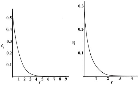
Fig. 3-4. The wave function and probability distribution as functions of r for the n = 1 level of the H atom. The functions and the radius r are in atomic units in this and succeeding figures.

Two interpretations can again be given to the P₁ curve. An experiment designed to detect the position of the electron with an uncertainty much less than the diameter of the atom itself (using light of short wavelength) will, if repeated a large number of times, result in Fig. 3-4 for P₁. That is, the electron will be detected close to the nucleus most frequently and the probability of observing it at some distance from the nucleus will decrease rapidly with increasing r. The atom will be ionized in making each of these observations because the energy of the photons with a wavelength much less than 10^-8 cm will be greater than K, the amount of energy required to ionize the hydrogen atom. If light with a wavelength comparable to the diameter of the atom is employed in the experiment, then the electron will not be excited but our knowledge of its position will be correspondingly less precise. In these experiments, in which the electron's energy is not changed, the electron will appear to be "smeared out" and we may interpret P₁ as giving the fraction of the total electronic charge to be found in every small volume element of space. (Recall that the addition of the value of P_n for every small volume element over all space adds up to unity, i.e., one electron and one electronic charge.)

    When the electron is in a definite energy level we shall refer to the P_n distributions as electron density distributions, since they describe the manner in which the total electronic charge is distributed in space. The electron density is expressed in terms of the number of electronic charges per unit volume of space, e^-/V. The volume V is usually expressed in atomic units of length cubed, and one atomic unit of electron density is then e^-/a₀³. To give an idea of the order of magnitude of an atomic density unit, 1 au of charge density e^-/a₀³ = 6.7 electronic charges per cubic Ångstrom. That is, a cube with a length of  0.52917 ´10^-8 cm, if uniformly filled with an electronic charge density of 1 au, would contain 6.7 electronic charges.

    P₁ may be represented in another manner. Rather than considering the amount of electronic charge in one particular small element of space, we may determine the total amount of charge lying within a thin spherical shell of space. Since the distribution is independent of direction, consider adding up all the charge density which lies within a volume of space bounded by an inner sphere of radius r and an outer concentric sphere with a radius only infinitesimally greater, say r + Dr. The area of the inner sphere is 4pr² and the thickness of the shell is Dr. Thus the volume of the shell is 4pr² Dr (Click here for note.) and the product of this volume and the charge density P₁(r), which is the charge or number of electrons per unit volume, is therefore the total amount of electronic charge lying between the spheres of radius r and r + Dr. The product 4pr²P_n is given a special name, the radial distribution function, which we shall label Q_n(r).

The radial distribution function is plotted in Fig. 3-5 for the ground state of the hydrogen atom.

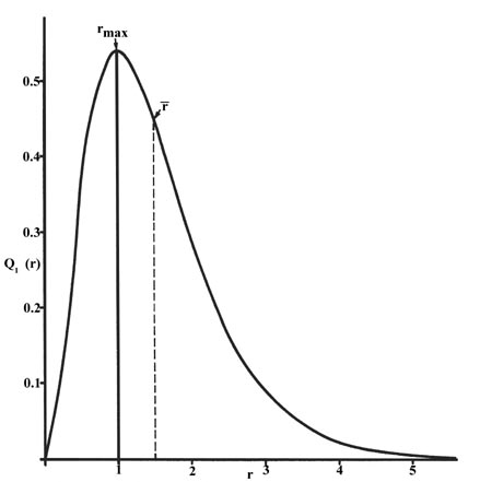Fig. 3-5. The radial distribution function Q1(r) for an H atom. The value of this function at some value of r when multiplied by Dr gives the number of electronic charges within the thin shell of space lying between spheres of radius r and r + Dr.

  The curve passes through zero at r = 0 since the surface area of a sphere of zero radius is zero. As the radius of the sphere is increased, the volume of space defined by 4pr²Dr increases. However, as shown in Fig 3-4, the absolute value of the electron density at a given point decreases with r and the resulting curve must pass through a maximum. This maximum occurs at r_max = a₀. Thus more of the electronic charge is present at a distance a₀, out from the nucleus than at any other value of r. Since the curve is unsymmetrical, the average value of r, denoted by , is not equal to r_max. The average value of r is indicated on the figure by a dashed line. A "picture" of the electron density distribution for the electron in the n = 1 level of the hydrogen atom would be a spherical ball of charge, dense around the nucleus and becoming increasingly diffuse as the value of r is increased.

    We could also represent the distribution of negative charge in the hydrogen atom in the manner used previously for the electron confined to move on a plane, Fig. 2-4, by displaying the charge density in a plane by means of a contour map. Imagine a plane through the atom including the nucleus. The density is calculated at every point in this plane. All points having the same value for the electron density in this plane are joined by a contour line (Fig. 3-6). Since the electron density depends only on r, the distance from the nucleus, and not on the direction in space, the contours will be circular. A contour map is useful as it indicates the "shape" of the density distribution.

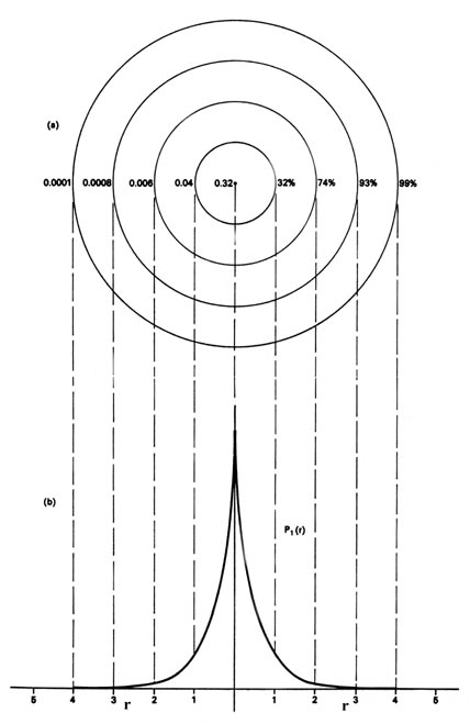Fig. 3-6.  (a) A contour map of the electron density distribution in a plane containing the nucleus for the n = 1 level of the H atom. The distance between adjacent contours is 1 au. The numbers on the left-hand side on each contour give the electron densityin au. The numbers on the right-hand side give the fraction of the total electronic charge  which lies within a sphere of that radius. Thus 99% of the single electronic charge of the H atom lies within a sphere of radius 4 au (or diameter = 4.2 ´10-8 cm). (b) This is a profile of the contour map along a line through the nucleus. It is, of course, the same as that given previously in Fig. 3-4 for P1, but now plotted from the nucleus  in both directions.

This completes the description of the most stable state of the hydrogen atom, the state for which n = 1. Before proceeding with a discussion of the excited states of the hydrogen atom we must introduce a new term. When the energy of the electron is increased to another of the allowed values, corresponding to a new value for n, y_n and P_n change as well. The wave functions y_n for the hydrogen atom are given a special name, atomic orbitals, because they play such an important role in all of our future discussions of the electronic structure of atoms. In general the word orbital is the name given to a wave function which determines the motion of a single electron. If the one-electron wave function is for an atomic system, it is called an atomic orbital. (Click here for note.)

    For every value of the energy E_n, for the hydrogen atom, there is a degeneracy equal to n². Therefore, for n = 1, there is but one atomic orbital and one electron density distribution. However, for n = 2, there are four different atomic orbitals and four different electron density distributions, all of which possess the same value for the energy, E₂. Thus for all values of the principal quantum number n there are n² different ways in which the electronic charge may be distributed in three-dimensional space and still possess the same value for the energy. For every value of the principal quantum number, one of the possible atomic orbitals is independent of direction and gives a spherical electron density distribution which can be represented by circular contours as has been exemplified above for the case of n = 1. The other atomic orbitals for a given value of n exhibit a directional dependence and predict density distributions which are not spherical but are concentrated in planes or along certain axes. The angular dependence of the atomic orbitals for the hydrogen atom and the shapes of the contours of the corresponding electron density distributions are intimately connected with the angular momentum possessed by the electron.

    The physical quantity known as angular momentum plays a dominant role in the understanding of the electronic structure of atoms. To gain a physical picture and feeling for the angular momentum it is necessary to consider a model system from the classical point of view. The simplest classical model of the hydrogen atom is one in which the electron moves in a circular orbit with a constant speed or angular velocity (Fig. 3-7). Just as the ordinary momentum mv plays a dominant role in the analysis of straight line or linear motion, so angular momentum plays the central role in the analysis of a system with circular motion as found in the model of the hydrogen atom.

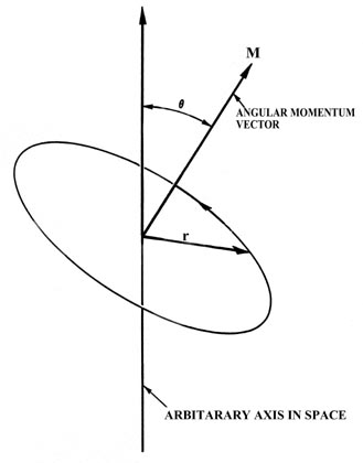
Fig. 3-7. The angular momentum vector for a classical model of the atom.

In Fig. 3-7, m is the mass of the electron, v is the linear velocity (the velocity the electron would possess if it continued moving at a tangent to the orbit as indicated in the figure) and r is the radius of the orbit. The linear velocity v is a vector since it possesses at any instant both a magnitude and a direction in space. Obviously, as the electron rotates in the orbit the direction of v is constantly changing, and thus the linear momentum mv is not constant for the circular motion. This is so even though the speed of the electron (the magnitude of v which is denoted by u) remains unchanged. According to Newton's second law, a force must be acting on the electron if its momentum changes with time. This is the force which prevents the electron from flying on tangent to its orbit. In an atom the attractive force which contains the electron is the electrostatic force of attraction between the nucleus and the electron, directed along the radius r at right angles to the direction of the electron's motion.

    The angular momentum, like the linear momentum, is a vector and is defined as follows:
 

The angular momentum vector M is directed along the axis of rotation. From the definition it is evident that the angular momentum vector will remain constant as long as the speed of the electron in the orbit is constant (u remains unchanged) and the plane and radius of the orbit remain unchanged. Thus for a given orbit, the angular momentum is constant as long as the angular velocity of the particle in the orbit is constant. In an atom the only force on the electron in the orbit is directed along r; it has no component in the direction of the motion. The force acts in such a way as to change only the linear momentum. Therefore, while the linear momentum is not constant during the circular motion, the angular momentum is. A force exerted on the particle in the direction of the vector v would change the angular velocity and the angular momentum. When a force is applied which does change M, a torque is said to be acting on the system. Thus angular momentum and torque are related in the same way as are linear momentum and force.

    The important point of the above discussion is that both the angular momentum and the energy of an atom remain constant if the atom is left undisturbed. Any physical quantity which is constant in a classical system is both conserved and quantized in a quantum mechanical system. Thus both the energy and the angular momentum are quantized for an atom.

There is a quantum number, denoted by l, which governs the magnitude of the angular momentum, just as the quantum number n determines the energy. The magnitude of the angular momentum may assume only those values given by:
 

(4)

Furthermore, the value of n limits the maximum value of the angular momentum as the value of l cannot be greater than n - 1. For the state n = 1 discussed above, l may have the value of zero only. When n = 2, l may equal 0 or 1, and for n = 3, l = 0 or 1 or 2, etc. When l = 0, it is evident from equation (4) that the angular momentum of the electron is zero. The atomic orbitals which describe these states of zero angular momentum are called s orbitals. The s orbitals are distinguished from one another by stating the value of n, the principal quantum number. They are referred to as the 1s, 2s, 3s, etc., atomic orbitals.

    The preceding discussion referred to the 1s orbital since for the ground state of the hydrogen atom n = 1 and l = 0. This orbital, and all s orbitals in general, predict spherical density distributions for the electron as exemplified by Fig. 3-5 for the 1s density. Figure 3-8 shows the radial distribution functions Q(r) which apply when the electron is in a 2s or 3s orbital to illustrate how the character of the density distributions change as the value of n is increased. (Click here for note.)

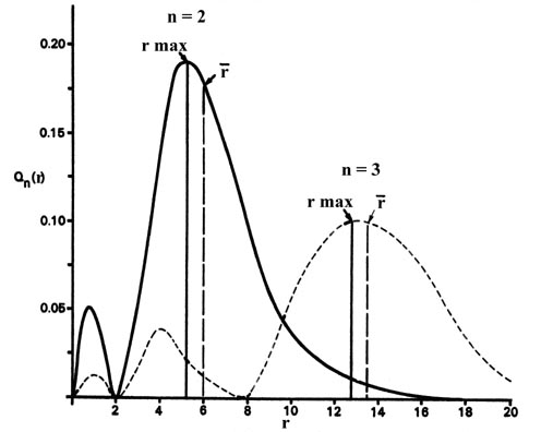
Fig. 3-8. Radial distribution functions for the 2s and 3s density distributions.

Comparing these results with those for the 1s orbital in Fig. 3-5 we see that as n increases the average value of r increases. This agrees with the fact that the energy of the electron also increases as n increases. The increased energy results in the electron being on the average pulled further away from the attractive force of the nucleus. As in the simple example of an electron moving on a line, nodes (values of r for which the electron density is zero) appear in the probability distributions. The number of nodes increases with increasing energy and equals n - 1.

When the electron possesses angular momentum the density distributions are no longer spherical. In fact for each value of l, the electron density distribution assumes a characteristic shape (Fig. 3-9).

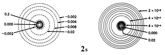
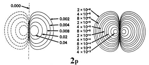
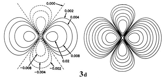
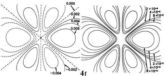
Fig. 3-9. Contour maps of the 2s, 2p, 3d and 4f atomic orbitals and their charge density distributions for the H atom. The zero contours shown in the maps for the orbitals define the positions of the nodes. Negative values for the contours of the orbitals are indicated by dashed lines, positive values by solid lines.

When l = 1, the orbitals are called p orbitals. In this case the orbital and its electron density are concentrated along a line (axis) in space. The 2p orbital or wave function is positive in value on one side and negative in value on the other side of a plane which is perpendicular to the axis of the orbital and passes through the nucleus. The orbital has a node in this plane, and consequently an electron in a 2p orbital does not place any electronic charge density at the nucleus. The electron density of a 1s orbital, on the other hand, is a maximum at the nucleus. The same diagram for the 2p density distribution is obtained for any plane which contains this axis. Thus in three dimensions the electron density would appear to be concentrated in two lobes, one on each side of the nucleus, each lobe being circular in cross section (Fig. 3-10).

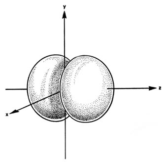
Fig. 3-10. The appearance of the 2p electron density distribution in three-dimensional space.

When l = 2, the orbitals are called d orbitals and Fig. 3-9 shows the contours in a plane for a 3d orbital and its density distribution. Notice that the density is again zero at the nucleus and that there are now two nodes in the orbital and in its density distribution. As a final example, Fig. 3-9 shows the contours of the orbital and electron density distribution obtained for a 4f atomic orbital which occurs when n = 4 and l = 3. (Click here for note.) The point to notice is that as the angular momentum of the electron increases, the density distribution becomes increasingly concentrated along an axis or in a plane in space. Only electrons in s orbitals with zero angular momentum give spherical density distributions and in addition place charge density at the position of the nucleus.

    We have not as yet accounted for the full degeneracy of the hydrogen atom orbitals which we stated earlier to be n² for every value of n. For example, when n = 2, there are four distinct atomic orbitals. The remaining degeneracy is again determined by the angular momentum of the system. Since angular momentum like linear momentum is a vector quantity, we may refer to the component of the angular momentum vector which lies along some chosen axis. For reasons we shall investigate, the number of values a particular component can assume for a given value of l is (2l + 1). Thus when l = 0, there is no angular momentum and there is but a single orbital, an s orbital. When l = 1, there are three possible values for the component (2´ 1 + 1) of the total angular momentum which are physically distinguishable from one another. There are, therefore, three p orbitals. Similarly there are five d orbitals, (2 ´ 2+1), seven f orbitals, (2 ´ 3 +1), etc. All of the orbitals with the same value of n and l, the three 2p orbitals for example, are similar but differ in their spatial orientations.

To gain a better understanding of this final element of degeneracy, we must consider in more detail what quantum mechanics predicts concerning the angular momentum of an electron in an atom.