An Introduction to the Electronic Structure of Atoms and Molecules

    Since the nuclear charge is twice the electronic charge, the electrostatic energy of repulsion between the electrons will be the smallest of the three terms in equation (1) when the interactions are averaged over all possible positions of the electrons. We could obtain an approximation to the electronic energy of the He atom by neglecting this small term. This is a good idea for another reason. If we ignore the repulsion between the electrons, then physically we are supposing that neither electron "realizes" the other electron is present. The problem is thus identical to that of the hydrogen atom, a problem which can be solved exactly, except that the nuclear charge is now +2 rather than +1.

    The energy of each electron in the field of a nucleus of charge +2 is determined separately and the total energy is then simply the sum of the two energies. This is the first approximation to the energy. We will also obtain an approximation to the manner in which the electrons are distributed in space. With this latter knowledge, we can estimate the energy of repulsion between the electrons. That is, with the knowledge of how the electrons are distributed relative to one another we can pick up the term in the potential energy we originally neglected, the term e²/r₁₂, and calculate its contribution to the energy.

   This method of calculating the electronic energy of atoms reduces a many-electron problem to many one-electron problems. Each electron (moving in the attractive field of the nucleus) is treated independently of the others. In addition, since the problem is now a set of one-electron problems, we may carry over and use all of the results obtained for the hydrogen atom.

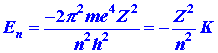
   We pointed out in our discussion of the hydrogen atom that the results we obtained could be applied to any one-electron system by setting Z equal  to the appropriate value in all of the formulae. The one-electron energies are easily calculated and are given by . More important, the concept of atomic orbitals, the one-electron wave functions for the hydrogen atom, may be employed in the many-electron case. When each electron is considered in turn, its motion and distribution in space will again be determined by an atomic orbital. The atomic orbitals will differ from the case of  the hydrogen atom in that they will generally be more contracted  In the previous chapter we pointed out that the average value of the distance between the nucleus and the electron, , decreased as the nuclear charge and hence the attractive force exerted by the nucleus was increased However, the orbitals will still be determined by the three quantum numbers n, l and m. Increasing Z contracts the orbital, but the symmetry of the problem  is left unchanged, i.e., the attraction of the electron by the nucleus is still determined only by the distance between them and does not depend on the direction.

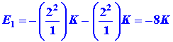
    The l and m dependences of the orbitals, which determine the directional properties of the orbital and of the electron density distribution, remain unchanged. Thus we may still refer to "hydrogen-like" 1s, 2s, 2p orbitals For example, the 1s orbital is the most stable orbital (most negative E value) for any value of Z, and we naturally assume that the most stable form of the helium atom will be obtained when both electrons are placed in the 1s orbital. This information, telling us in which atomic orbital the electrons have been placed, is called an electron configuration.

   An abbreviated notation is used to denote the electron configuration For example, the lowest energy state of helium, in which two electrons are placed in the 1s orbital, is written as 1s². (This is to be read as one-s-two and not as one-s-squared.) When one of the electrons is placed in an orbital of higher energy, an "excited" configuration is obtained. An example might be 1s¹2p¹ which one electron is in the 1s orbital and one electron is in the 2p orbital. It should be emphasized that the concept of assigning an electronto an atomic orbital is a rigorous and exact concept only for the hydrogen atom; for the many-electron case it is an approximation.

   The atomic orbital approximation may be tested by applying it to the helium atom. We have seen that the energy of a single electron moving in the attractive field of a nucleus of charge +Ze is
 

(2)

The energy of the two electrons in the helium atom, each considered to be independent of the other, is simply
 

for the 1s² electron configuration. To this energy value must be added the energy of replusion between the two electrons. Since both electrons have been placed in a 1s atomic orbital, we know that the charge distribution for each electron must be spherical and centred on the helium nucleus. The two charge distributions will be completely intermingled and we must calculate the energy of replusion between every small element of charge density of the one distribution with every small charge element of the second distribution. This calculation can be readily done by the methods of integral calculus and the value of the average energy replusion is found to be
 

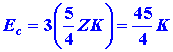
We label this energy E_c as it is a correction to our first approximation to the energy. Notice that in general E_c depends directly on the value of Z. This makes physical sense, for the greater the value of Z, the more contracted and superimposed are the two charge distributions, and the greater is the energy of replusion between them. Note as well that the correction E_c is indeed smaller than E₁, an assumption we made in developing this method of approximating the electronic energy.

   The estimate of the total electronic energy of helium atom is
 

This total energy is called the electronic binding energy as it is the energy released when two initially free electrons are bound to the helium nucleus Recall that -K represents the binding energy of the most stable state of the hydrogen atom; thus the helium atom is five and one half times more stable than the hydrogen atom. This is not really a fair comparison because the value (11/2)K is the energy required to remove both electrons from the helium atom (a double ionization)
 

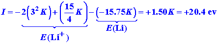
It is more interesting to compare the energy required to remove a single electron from helium with the energy required to remove the single electron in hydrogen. The energy of the reaction (The energy required to ionize an atom will be denoted by the letter I.)
 

is easily caluclated
 

The energy of the He⁺  ion using equation (2) with n = 1 and Z = 2, is
 

as there is but a single electron left. The energy of the ionized electron E_e- is set equal to zero as it is assumed to be at rest infinitely far away from the ion and E_He =  -(11/2)K. Thus I, the first ionization potential of helium, is equal to 1.5K, or one and one half times larger than the energy required to ionize a hydrogen atom.

  How well do our calculated values for the ionization potential and total energy agree with the experimental results? The energy required for the removal of both electrons is 78.98 ev. Since K = 13.61 ev, the calculated value is (11/2)13.61 = 74.86 ev. This is an encouraging result as the error is only about 5%. The experimental value for I is 24.58 ev and our calculated value is (1.5)13.61 = 20.42 ev. The percentage error is larger for the latter case because the actual error is the same in both calculations but I is smaller than DE. However, the method seems promising. We have indeed predicted that it requires almost twice as much energy to remove an electron from helium as it does to remove one from hydrogen.

   The calculations outlined above may be improved by introducing the concept of an effective nuclear charge. Since there are two electrons present in the helium atom, neither electron experiences the full attractive force of the two positive charges on the helium nucleus. Each electron partially screens the nuclear charge from the other. We saw previously that the averagevalue of the distance between an electron and the nucleus for a strictly hydrogen-like orbital varied as (1/Z). Thus by assuming that each electron moves in the field of the full nuclear charge of helium, we consider it to be in a 1s orbital with exactly one half the value of  as that found for a hydrogen 1s orbital. Since the electron on the average experiences a rereduced nuclear charge (i.e., the effective nuclear charge) because of the screening effect of the second electron, we should place it in a 1s orbital which possesses an  value somewhere between that found for an orbital for the cases Z = 1 and Z = 2. In other words, the size of the orbital should be determined by an effective nuclear charge, rather than by the actual nuclear charge. This lowered value for Z will obviously decrease the value of the average repulsion energy between the electrons as the two charge clouds will be more expanded and the average distance between the charge points in each distribution will increase. An increased value of will also decrease the average kinetic energy of the electrons and thus again lead to an increase in the stability of the atom. On the other hand, an increase in  will lead to a less negative potential energy as the electrons will on the average be further away from the nucleus. Thus there is some best value for the effective nuclear charge and for , the value which gives the most stable description of the atom. For helium this "best" value for the effective nuclear charge is found to be 1.687 and the total energy of He is now  calculated to be 77.48 ev. The error has been reduced to approximately 2%.

   The effective nuclear charge value cannot be inserted into equation (2) to determine the energy of the electron. The Z in equation (2) refers to the actual nuclear charge, while the effective nuclear charge is a number, always less than the actual Z. which determines the optimum size of the orbital when other electrons are present. The value of Z appearing in the equate for E_c will be the effective nuclear charge value. The value of E_c is indeed determined solely by the degree to which the two electron distributions are contracted and this is governed by the effective nuclear charge. It should be pointed out that the concept of an effective nuclear charge will be paramount  in our future discussions concerning the electronic structures and properties of many-electron atoms.

Excited states of the helium atom.  Just as the single electron in the hydrogen atom can be excited to higher quantum levels, so it should be possible to excite one of the electrons in the He atom to energy levels with quantum numbers greater than one. This will change the electron configuration from 1s² to say, ls¹2s¹ or 1s¹2p¹ etc. The excited electron may again lose the excitation energy in the form of light and fall back to the 1s level, giving the ground electronic configuration 1s²
 

Thus the helium atom should emit a line spectrum when it is excited in an electrical discharge tube. Since only a single electron is excited at a given  time although if is possible with the use of a laser to excite two electrons simultanously-the spectrum for helium should be formally the same as that observed for hydrogen. However, since the nuclear charge experienced by the electron will always be greater than one, the lines in the helium spectrum should be observed at higher frequencies (shorter wavelengths) than those for hydrogen.

In Table 4-1. we compare two corresponding line spectra, one for hydrogen and one from helium. In both cases the excited electron fall from an upper p energy level to the 2s energy level. In hydrogen the frequencies of the lines in the spectrum are determined by the energy differences between the configuration.
 

       This series of jumps from E_n (n = 3, 4, 5, 6, . . . ) to E₂ level generates the Balmer series of lines which we discussed earlier. We are now being more specific in stating that in this particular examples the excited electrons in in an np orbital. The helium spectrum we wish to compare with this one arises from the transition between configurations
 

Qualitatively the two spectra are the same, as our model predicted. In addition, the helium lines occur at shorter wavelengths (higher energies) than for hydrogen. In fact, for every series of lines (Lyman, Balmer, etc.) found for hydrogen, there is a corresponding series found at shorter wavelengths for helium. Our model, which uses hydrogen-like atomic orbitals to describe many-electron atoms, looks promising indeed. However, it is in the study of the spectrum of helium that we encounter the first shortcoming of this simple approach; there are two series of lines observed for helium for every single series of lines observed for hydrogen. Not only does helium possess the "Balmer" series quoted in Table 4-1, it has a second "Balmer"series starting at l = 3889A. That is, the whole series is repeated at shorter wavelengths. Rather than abandon the atomic orbital approach for the many-electron atom, let us keep the above failure of the method in mind and proceed with an application to the lithium atom.

The lithium atom.  There are three electrons in the lithium atom (Z = 3) but the total repulsion energy between the electrons is still determined by considering the repulsions between a pair of electrons at a time. For this reason, three electrons are fundamentally no more difficult to treat than two electrons. There are simply more possible pairs and hence more repulsive interactions to consider than in the two-electron case. The dependence of the potential energy on the distances between the electrons and between the electrons and the nucleus is
 

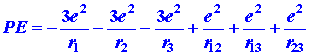where r₁₂, is the distance between electrons 1 and 2, r₁₃ the distance between electrons 1 and 3, and r₂₃ the distance between electrons 2 and 3.

   It is natural to assume that, as in the case of hydrogen or helium, the most stable energy of the lithium atom will be obtained when all three electrons are placed in the 1s atomic orbital giving the electronic configuration 1s³. Proceeding as in the case of helium we calculate the first approximation to the energy to be (using equation (2))
 

This represents the sum of the energies obtained when each electron is considered to move independently in the field of the nucleus of charge +3 in an orbital with n = 1. To this must be added the energy of repulsion between the electrons. The average repulsion energy between a pair of electrons is again given by . In lithium we must consider the repulsion between electrons 1 and 2, between electrons 1 and 3, and between electrons 2 and 3. Therefore the total repulsion energy which represents the correction to E is
 

and the total electronic energy of the lithium atom is predicted to be
 

Thus it should require 214.4 ev to remove all three electrons from the lithium atom.

    We can also calculate the energy required to remove a single electron from  lithium (the first ionization potential)
 

       When the predicted values for lithium are compared with the corresponding experimental values, they are found to be in serious error. The lithium atom is not as stable as the calculations would suggest. Experimentally it requires 202.5 ev to remove all three electrons from lithium, and only 5.4 ev to remove one electron. Experimentally it requires less energy to ionize lithium than it does to ionize hydrogen, yet our calculation predicts an ionization energy one and one half times larger. The error in I is 300%! We should expect a realistic model to do better than this. More serious than this, however, is that the kind of calculation we are doing should never predict the system to be more stable than it actually is. The method should always predict an energy less negative than is actually observed. If this is not  found to be the case, then it means that an incorrect assumption has been made or that some physical principle has been ignored. It is also clear that if we were to continue this scheme of placing each succeeding electron in the 1s orbital as we increased the nuclear charge by unity we would never predict the most striking property of the elements:  the property of periodicity.

    We might recall at this point that there is a periodicity in the types of atomic orbitals found for the hydrogen atom. With every increase in n, all the preceding values of l are repeated, and a new l value is introduced. If we could discover a physical reason for not placing all of the electrons in the1s orbital, but instead place succeeding electrons in the orbitals with higher n values, we could expect to obtain a periodicity in our predicted electronic structures for the atoms. This periodicity in electronic structure would then explain the observed periodicity in their properties. There must be another factor governing the behaviour of electrons and this factor must be one which determines the number of electrons that may be accommodated in a given orbital. To discover what this missing factor is and to find the physical basis for it, we must investigate further the magnetic properties of electrons.